Google Sheets is rich with hidden tips and tricks that can not only speed up your workflow, but also add some oomph to the way you present data. And while Google Sheets isn’t necessarily as powerful as Microsoft’s Excel, the fact that it is free means it is the go-to solution for many users who don’t need all the might of Excel.

Google doesn’t release details of monthly-active users, but an independent analysis by SurveyMonkey in 2016 showed that Google Sheets significantly outperforms Excel — at least on mobile. And if you happen to use Google Sheets on a regular basis, you’re bound to appreciate some of the tips and tricks listed below.

1. Conditional Formatting With Heatmaps

Any spreadsheet collecting together large amounts of data can benefit from conditional formatting to highlight specific bits of data. But by applying a Color Scale to your conditional formatting, you can emulate a heatmap, with different shades of the same colour (or your own custom colour scale) highlighting high and low values, so it is easier to identify which data to focus on.

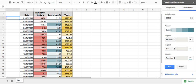
This can be especially useful when analysing performance metrics.

2. Use the Trim and Clean Functions

Whenever you import data from another source, and this data (text or numbers) is going to be used in formulas, it is wise to use TRIM and CLEAN to remove leading and trailing spaces, along with any non-printable characters. Leading spaces are easy to notice, but trailing spaces and non-printable characters are not: Google Sheets does not display non-printable characters. If you are not sure whether you should be cleaning or trimming, combine the two as shown in the image below.

Now you can copy the cleaned and trimmed data, and using Paste special, paste as values only in a new row or column, and continue with your work.

3. Collect Survey Responses

This tip doesn’t apply to a broad range of users, but if you happen to use Google Forms to draw up surveys, job applications, etc. you can have all responses automatically sent to a new or existing Google Sheet.

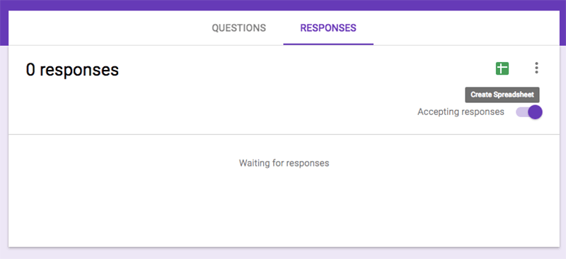
After you have created your Google Form, select the Responses tab, and then select the Google Sheets icon in the panel that is revealed. You will now have an opportunity to name and create a new sheet, or select an existing sheet. Creating a new sheet opens the new sheet in Google Sheets, with a Timestamp column, and columns for each of the questions in your form.

4. Import Data From Other Sheets, Websites, and RSS Feeds

The IMPORT function can be used to import data from other sheets, websites, or RSS feeds, saving you loads of time in the process. This function supports the following commands:

• • IMPORTHTML: Imports data from a table or list within an HTML page.

• • IMPORTXML: Imports data from any of various structured data types including XML, HTML, CSV, TSV, and RSS and ATOM XML feeds.

• • IMPORTRANGE: Imports a range of cells from a specified spreadsheet.

• • IMPORTFEED: Imports a RSS or ATOM feed.

• IMPORTDATA: Imports data at a given url in .csv (comma-separated value) or .tsv (tab-separated value) format.

The syntax varies for each, so it is important to familiarise yourself with them using the Google Help documents linked above.

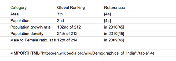
The image above shows the syntax — and result — for using IMPORTHTML.

5. Translate Text

Another tip not called for frequently, but you’ll be happy it exists if you ever need it. Google Docs embraced online collaboration long before Microsoft Office did, so there’s always a chance you’ll be working with people in other locations, leading to data that is entered or provided in a different language. When this happens, simply use the =GOOGLETRANSLATE function to automatically translate the text into your preferred language.

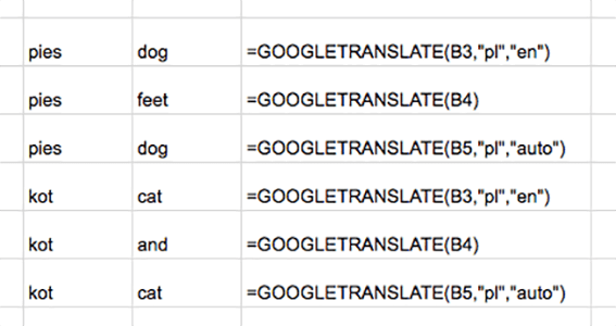
Unfortunately, Google Translate won’t always pick up the correct source language correctly, so you can avoid further mistakes by specifying the source or target language (or both), using the relevant two letter language codes (ISO 639–1 codes).

6. Split Data

Adding data from a CSV file will sometimes separate nicely in Google Sheets, and others times not at all. And for those times that it doesn’t, the Split text to columns function can be a life saver. But that function doesn’t only work for comma separated values; it can also be used on data separated by semicolons, periods, spaces, or any custom element of your choosing.

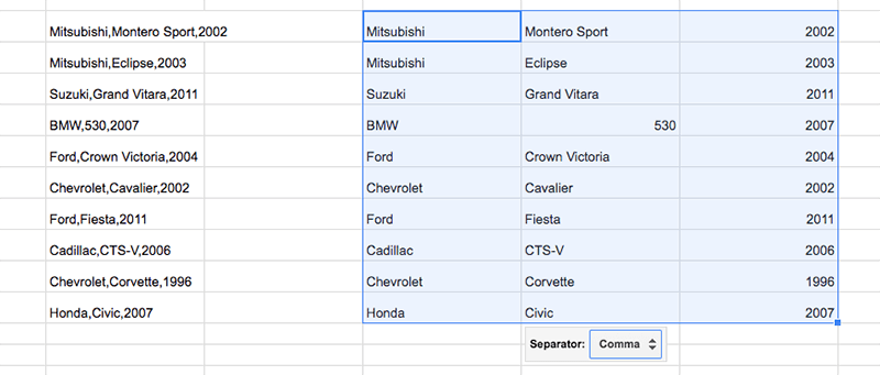
Splitting car makes, models, and years into individual columns is easy when they’re separated by a comma, less so when they’re separated by a space. The Split text to columns function can be found under the Data menu tab.

7. Use Sparklines to Visualise Your Data

Sparklines are a nifty way to visualise trends when a full-sized chart isn’t called for. And using the =SPARKLINE function, you can easily add a sparkline anywhere in your Google Sheet, for any bits of data.

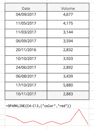
The list of possible syntax options is quite long for sparklines, with options to not only specify the chart type, but also colour, line width, and even how to treat empty cells, or cells with non-numeric data.

8. Add Data Validation Rules

The collaborative nature of spreadsheets means at times you will need to share a sheet with other people — for them to input their own data. Which exposes you to the risk of data that is added incorrectly. And we’re not just talking about a typo or two; we’re talking people adding “twenty” instead of “20”, or “35%” instead of just “35”. You can avoid this by adding data validation rules to specific cells, forcing data to only be added in certain formats.

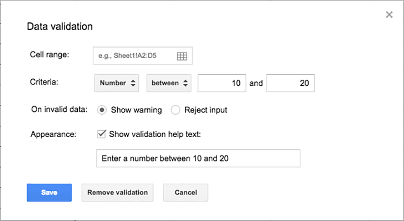
Data validation is the last option under the Data menu tab, and you can set various criteria including:

• • Lists — from a range, or comma separated items you add yourself.

• • Numbers

• • Text

• • Dates

• Custom formula

You can also specify whether invalid data will be rejected, or just result in a warning, and also include help text if you want.

9. Call up all Keyboard Shortcuts

Like most software, Google Sheets includes numerous keyboard shortcuts that can help speed up your workflow. But if you’re anything like me, you only remember a handful of the most commonly used shortcuts. Use cmd + / (⌘ + / ) on a Mac, or ctrl + / on Windows, to bring up a neatly arranged list of all possible keyboard shortcuts for Google Sheets, along with the ability to override browser shortcuts.

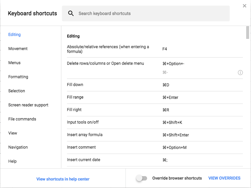
There are also shortcuts available for when you’re working on a mobile device, though shortcuts for iOS are quite limited.

10. Add Charts to Your Google Docs

Finally, adding a chart you have created in Google Sheets to Google Docs used to rely on an add-on. But now you can do this without first having to visit the Chrome web store. Navigate to Insert > Chart in the Google Docs you are working on, and you will now see a From Sheets option. This will present you with a view of all your Google Sheets (personal, and those shared with you). Note that you will get an error message if you select a Sheet that doesn’t have any charts already. And any changes you make to the data used to create the chart will see the chart in your Google Docs update automatically, so there’s no need to manually maintain two charts anymore.